

Codely v2.0 public release is here
Lorem ipsum dolor sit amet, consectetur adipiscing elit lobortis arcu enim urna adipiscing praesent velit viverra sit semper lorem eu cursus vel hendrerit elementum morbi curabitur etiam nibh justo, lorem aliquet donec sed sit mi dignissim at ante massa mattis.
- Neque sodales ut etiam sit amet nisl purus non tellus orci ac auctor
- Adipiscing elit ut aliquam purus sit amet viverra suspendisse potent i
- Mauris commodo quis imperdiet massa tincidunt nunc pulvinar
- Adipiscing elit ut aliquam purus sit amet viverra suspendisse potenti
What has changed in our latest release?
Vitae congue eu consequat ac felis placerat vestibulum lectus mauris ultrices cursus sit amet dictum sit amet justo donec enim diam porttitor lacus luctus accumsan tortor posuere praesent tristique magna sit amet purus gravida quis blandit turpis.
All new features available for all public channel users
At risus viverra adipiscing at in tellus integer feugiat nisl pretium fusce id velit ut tortor sagittis orci a scelerisque purus semper eget at lectus urna duis convallis. porta nibh venenatis cras sed felis eget neque laoreet suspendisse interdum consectetur libero id faucibus nisl donec pretium vulputate sapien nec sagittis aliquam nunc lobortis mattis aliquam faucibus purus in.
- Neque sodales ut etiam sit amet nisl purus non tellus orci ac auctor
- Adipiscing elit ut aliquam purus sit amet viverra suspendisse potenti
- Mauris commodo quis imperdiet massa tincidunt nunc pulvinar
- Adipiscing elit ut aliquam purus sit amet viverra suspendisse potenti
Coding collaboration with over 200 users at once
Nisi quis eleifend quam adipiscing vitae aliquet bibendum enim facilisis gravida neque. Velit euismod in pellentesque massa placerat volutpat lacus laoreet non curabitur gravida odio aenean sed adipiscing diam donec adipiscing tristique risus. amet est placerat in egestas erat imperdiet sed euismod nisi.
“Nisi quis eleifend quam adipiscing vitae aliquet bibendum enim facilisis gravida neque velit euismod in pellentesque massa placerat”
Real-time code save every 0.1 seconds
Eget lorem dolor sed viverra ipsum nunc aliquet bibendum felis donec et odio pellentesque diam volutpat commodo sed egestas aliquam sem fringilla ut morbi tincidunt augue interdum velit euismod eu tincidunt tortor aliquam nulla facilisi aenean sed adipiscing diam donec adipiscing ut lectus arcu bibendum at varius vel pharetra nibh venenatis cras sed felis eget dolor cosnectur drolo.
A manufacturing company is not worth just “EBITDA times a multiple.” I’d start with normalized earnings, check working capital, review equipment and customer risk, then bridge enterprise value to equity value. For example, $2,000,000 of normalized EBITDA at 5.0x points to $10,000,000 of enterprise value, but debt, cash, leases, tax items, and working-capital gaps can move the final price by hundreds of thousands of dollars.
Here’s the short version:
- I define what is being valued: the whole company, one plant, a division, or selected assets
- I clean up earnings to get normalized EBITDA or, for a very small owner-run shop, SDE
- I test inventory, receivables, payables, and capex, because EBITDA alone can overstate cash flow
- I use the right method: market, DCF/capitalized cash flow, or asset-based
- I adjust for risk, like:
- customer concentration
- old equipment
- labor issues
- compliance problems
- I convert enterprise value into equity value by adding cash and subtracting debt-like items
A few numbers stand out. The article notes 2025 manufacturing M&A EV/EBITDA data of about 5.7x to 9.5x, with an overall figure near 6.5x. It also shows how a $900,000 EBITDA business at 4.5x to 5.5x lands at about $4,050,000 to $4,950,000 in enterprise value before balance-sheet adjustments.
If I had to boil the process down, it would look like this:
| Step | What I check | Why it matters |
|---|---|---|
| 1 | Scope and valuation date | Keeps the model tied to the deal |
| 2 | Financials and plant data | Shows earnings quality and plant risk |
| 3 | Earnings adjustments | Removes owner-specific and one-time items |
| 4 | Working-capital target | Prevents cash shortfalls after closing |
| 5 | Valuation method | Matches the business to the right approach |
| 6 | EV-to-equity bridge | Turns headline value into actual seller proceeds |
Bottom line: I would treat the headline multiple as the start, not the answer. The final number should reflect earnings quality, equipment condition, working-capital needs, debt-like items, and the risk that future cash flow comes in below plan.
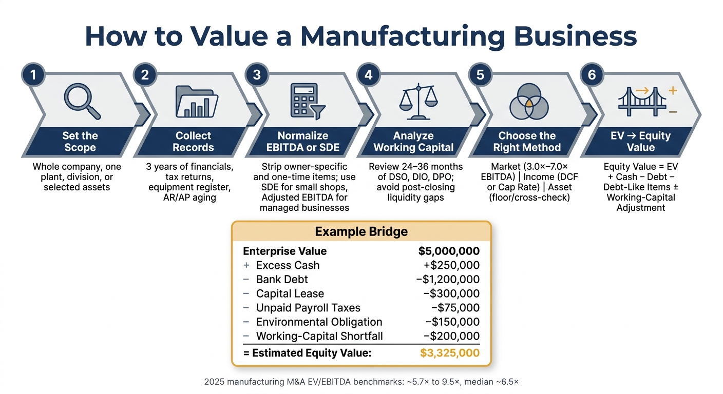
How to Value a Manufacturing Business: 6-Step Process
Gather Financial Statements and Plant-Level Operating Data
Once you’ve set the scope, the next step is simple: gather the records that support your earnings and balance-sheet adjustments.
Start with three years of annual financial statements, monthly financials for the last 12–24 months, and year-to-date results versus the same period last year. Annual statements give you the big picture. Monthly data shows what annuals often hide, like seasonality, margin changes, and working-capital swings. Add the general ledger and trial balance so you can trace revenue, expenses, owner pay, and add-backs back to actual entries. The point is to separate steady operating performance from noise and non-transferable items.
Next, collect three years of federal business tax returns and reconcile them line by line to the company-prepared statements. This helps you test revenue, depreciation, owner compensation, related-party payments, and taxable income. If something doesn’t match, flag it before it works its way into the model.
You’ll also want plant-level operating data. That means revenue by customer, segment margin, backlog detail, capacity use by production line, scrap and rework rates, and supplier concentration. This is where operating risk starts to show up in plain sight. Customer concentration can hit value hard, especially if a major customer can walk away at will.
For fixed assets, pull the full register: equipment description, acquisition date, original cost, accumulated depreciation, book value, and condition. Pair that with maintenance logs and inspection records. Book value tells you what’s on paper. It does not tell you how much life the equipment has left or whether a big replacement bill is around the corner. Also gather at least five years of capex history, split between maintenance and growth spending, plus the current capex budget.
Finally, collect AR and AP aging reports, inventory records, all debt and lease schedules, and any change-of-control terms in those agreements. These records help you spot debt-like items and hidden liabilities that can change equity value.
Use a Diligence Checklist Tied to Valuation Questions
Before you build the model, tie each document to a valuation question. If a document doesn’t help answer one, don’t spend time on it.
| Record | What it tests | Key follow-up question |
|---|---|---|
| Annual and monthly income statements | Revenue trend, margins, seasonality, earnings quality | Why did gross margin fall from 29% to 24%? |
| Balance sheets and cash-flow statements | Liquidity, leverage, working-capital intensity | Does reported cash flow support normalized EBITDA? |
| Federal tax returns | Reliability of reported earnings | Why does taxable revenue differ from book revenue? |
| AR aging | Collectability and working-capital needs | Which receivables are more than 90 days past due? |
| AP aging | Unrecorded liabilities and supplier pressure | Are overdue balances normal or a sign of liquidity pressure? |
| Inventory report and count records | Obsolescence, valuation, and turnover | What percentage hasn't moved in 12 months? |
| Fixed-asset register and maintenance logs | Equipment condition and remaining useful life | Which assets need replacement within three years? |
| Debt and lease schedules | Debt-like obligations and transaction adjustments | Which leases or loans require consent at closing? |
| Capex history and budget | Replacement-capex risk and future cash needs | How much of planned capex is maintenance rather than growth? |
| Revenue by customer and contracts | Concentration, retention, and pricing durability | Can the largest customer terminate without cause? |
| Gross margin by segment | Product and customer profitability | Is growth concentrated in a low-margin segment? |
| Backlog and capacity-utilization reports | Revenue visibility and operational constraints | Is backlog cancellable, profitable, and deliverable? |
| Supplier-spend analysis | Input-cost and continuity risk | Is there a qualified alternative supplier? |
| Labor, safety, and compliance records | Staffing, regulatory, and operational risk | Are margins dependent on overtime or deferred compliance work? |
Don’t stop at the documents.
A plant walkthrough, equipment inspection, and inventory observation help you compare the records to what’s actually happening on the floor. It’s one thing to read that scrap is low. It’s another to see bins of rework stacked near a line. Trace a few orders from raw material purchase through shipment. That kind of testing shows whether operating claims hold up in practice.
Use Kumo for Early Deal Screening, Not Final Valuation
If you’re sourcing manufacturing acquisition targets, Kumo can help at the sourcing stage. It pulls listings together, lets you filter targets, and makes it easy to export candidates for an initial pass.
That said, treat listing data as a starting point, not the answer. It helps you decide which targets deserve a closer look. After a target clears that first screen, use the diligence package above to build the valuation model.
sbb-itb-97ecd51
Normalize Earnings and Working Capital
Reported earnings almost never line up neatly with post-closing economics. That's why normalization matters. The goal is simple: strip out owner-specific and one-off items so you can see recurring earnings. That normalized figure then feeds the valuation methods that come next.
Seller's Discretionary Earnings (SDE) fits a small, owner-operated business where the buyer will step in and run the plant. It starts with net income, then adds back one owner's compensation and benefits, interest, taxes, depreciation, amortization, and documented personal or nonrecurring items. For a larger manufacturer with a management team - or for a buyer who won't be on the floor every day - adjusted EBITDA is the better tool. The big difference is that adjusted EBITDA keeps a market-rate management cost in place, while SDE does not. If you skip that cost, earnings look higher than they should. As a rough rule, the shift from SDE to EBITDA-based analysis often happens around $1 million to $1.5 million of normalized earnings, but the better test is owner involvement and management depth, not some fixed revenue line.
Build a recast schedule that covers at least three fiscal years, the trailing twelve months, and the current-year budget or forecast. Start with tax-return net income. Reconcile that to the financial statements. Then add back interest, taxes, depreciation, and amortization to arrive at reported EBITDA. After that, layer in documented normalization adjustments.
Adjusted EBITDA = reported EBITDA + defensible add-backs − nonrecurring gains and temporary benefits ± other normalization adjustments
This recast becomes the base for a market multiple or an income-based valuation.
Separate Legitimate Add-Backs From Ongoing Costs
Every add-back should clear three hurdles: it has source support, it's unusual or nonoperating, and it will not continue after closing. A documented legal settlement unrelated to normal operations can qualify. So can a one-time plant move or personal travel with no business purpose. On the other hand, recurring temporary labor, routine maintenance, normal warranty claims, ordinary freight swings, or any cost that shows up year after year should stay in the numbers, no matter how management describes it.
A good quality-of-earnings habit is to ask for source support for every proposed adjustment above $10,000 and to run a downside case where 30% of proposed add-backs don't materialize. Keep an add-back schedule that shows the general-ledger account for each item, the amount by period, why it qualifies, and the support behind it. Also flag any replacement cost. That part trips people up all the time. If an owner takes a $240,000 salary, that doesn't mean the full $240,000 is a clean add-back. If replacing that owner with a plant manager would cost $150,000, the defensible net adjustment is just $90,000.
Set a Normalized Working-Capital Target
Adjusted EBITDA can make cash flow look better than it is when working capital and capex are heavy. In manufacturing, working capital often carries a big chunk of the price story. A manufacturer showing $1,000,000 of adjusted EBITDA may still produce much less free cash flow once working capital, taxes, and maintenance capex are taken out.
Here is the basic bridge from adjusted EBITDA to operating cash flow:
| Reconciliation item | Treatment |
|---|---|
| Adjusted EBITDA | Starting normalized operating earnings |
| Cash taxes | Deduct taxes expected in normal operations |
| Change in accounts receivable | Deduct increases; declining receivables release cash |
| Change in inventory and WIP | Deduct increases across raw materials, WIP, and finished goods |
| Change in accounts payable and accrued liabilities | Add increases only when supplier timing is sustainable |
| Warranty, bonus, and other operating accruals | Adjust for cash paid versus expense recognized |
| Recurring capital expenditures | Deduct maintenance capex needed to keep the plant running |
| Free cash flow | Result after working-capital and recurring-investment requirements |
For the working-capital target, define operating working capital as accounts receivable plus inventory plus other operating current assets, minus accounts payable and other operating current liabilities. Leave out cash, debt, and income-tax accounts unless the purchase agreement says otherwise. Pull 24 to 36 months of monthly data. Then calculate days sales outstanding, days inventory outstanding, and days payable outstanding for each month. A year-end balance sheet can miss seasonality in a big way. If a manufacturer carries $2.4 million of working capital at peak production but only $1.5 million in the off-season, and closing happens before the seasonal build, the buyer could walk straight into a $900,000 liquidity shortfall right after closing.
Go deeper on inventory than the top-line balance. Review it by age, product family, and last usage date. Decent overall turns can still hide obsolete raw materials or finished goods that only move at a discount. For receivables, don't stop at the aging report. Test them against actual cash collected after the balance-sheet date. Then look at supplier payment timing. If the seller usually pays suppliers in 45 days but the closing balance reflects 75-day behavior, the working-capital target is too low, and the buyer will feel that gap on day one.
Each earnings metric has its own job:
| Metric | Definition | Best use case | Main limitation |
|---|---|---|---|
| SDE | Net income + one owner's compensation and benefits + interest + taxes + D&A + defensible nonrecurring items | Small, owner-operated businesses where the buyer runs the business | Can overstate transferable earnings if a replacement manager is needed |
| Adjusted EBITDA | EBITDA ± documented normalization adjustments, retaining market-rate management costs | Larger manufacturers with management teams or buyers who will not personally operate the business | Excludes working-capital investment, cash taxes, and capex |
| EBIT | Operating profit after depreciation and amortization, before interest and taxes | Asset-intensive businesses where depreciation reflects real economic wear | Sensitive to depreciation policy; doesn't measure cash generation |
| Free cash flow | EBITDA − cash taxes − Δ operating working capital − maintenance capex | Debt-capacity analysis and buyer return modeling | Requires careful assumptions about maintenance capex, taxes, and working capital |
Use SDE for very small owner-operated shops, adjusted EBITDA for managed businesses, EBIT for asset-heavy operations, and free cash flow to test debt capacity and purchase-price support.
Once earnings and working capital are normalized, the next move is to choose the valuation method that fits the business best.
Apply the Right Valuation Methods and Adjust for Manufacturing Risk
Once normalized earnings and working capital are set, the next step is choosing the valuation method that fits the business as it actually operates. That choice should line up with the risks found in the financial review and on the plant floor.
For a profitable manufacturer that will keep operating as a going concern, the biggest weight usually goes to normalized EBITDA or cash flow. But that changes when the company is underperforming, heavy on physical assets, or drifting toward liquidation. In those cases, machinery, tooling, inventory, and real estate may matter more.
Compare Market, Income, and Asset Approaches
The market approach applies observed transaction multiples to normalized EBITDA or another metric that fits the business. For privately held manufacturers, broad EBITDA multiples often land around 3.0×–7.0×, depending on subsector, size, and business quality. Use that range as a screening tool, not a final answer. Closed deals from the same subsector are far more useful than a generic industry multiple.
The income approach has two main forms. Discounted cash flow (DCF) works best when future cash flow is likely to look different from the past. That might happen when a company is installing an automated production line, moving into a new market, or losing a major program. Capitalized cash flow is simpler. It tends to fit a mature, stable manufacturer: take a sustainable normalized cash flow and divide it by a capitalization rate that reflects long-term growth and risk. DCF can move a lot with small changes in terminal growth, margins, or the discount rate, so sensitivity cases matter here.
The asset approach resets assets to fair market value or orderly liquidation value, then subtracts liabilities. In most manufacturing deals, that works better as a floor or cross-check than as a going-concern value.
| Approach | Best use case | Key limitation | Value indication |
|---|---|---|---|
| Market | A manufacturer with reliable comparable transactions and reasonably consistent earnings | Private-company data may be limited or hard to compare; headline multiples may reflect different debt, cash, or working-capital terms | Enterprise value based on an adjusted multiple |
| Income - DCF | A company with forecastable growth, changing margins, or identifiable investments | Very sensitive to growth, margins, terminal value, and discount rate assumptions | Present value of forecast and terminal cash flows |
| Income - Capitalized cash flow | A mature business with stable earnings, growth, and risk | Weak when earnings are volatile, cyclical, or expected to change in a major way | Capitalized value of a representative cash-flow level |
| Asset | Asset-heavy, distressed, low-profit, or liquidation-oriented manufacturers | May miss going-concern value tied to customers, workforce, know-how, and future earnings | Net asset value or liquidation-value floor |
The key point: weight the method that matches how a buyer gets paid back. Don’t just average the outputs. If the market approach points to $9.0 million to $11.0 million and a DCF backs up that range, but adjusted net assets come in at $6.5 million, the asset result is more of a downside marker. A sound conclusion might land at $9.5 million to $10.0 million and explain why the upper end was not used.
Adjust the Multiple for Customer, Equipment, Labor, and Compliance Risk
This is where diligence findings start to change the number. Plant conditions, customer mix, labor stability, and compliance issues all affect where a company falls within the valuation range. In plain English: the same manufacturer on paper can be worth more or less depending on what sits behind the numbers.
Customer concentration is one of the most common drags on value. The adjustment should reflect both the odds of losing the customer and the damage if that happens. So don’t stop at the concentration percentage. Look at contract length, switching costs, customer tenure, and past retention too. Recurring service, maintenance, or aftermarket revenue makes earnings easier to rely on and usually supports a stronger multiple.
Equipment condition matters for the same reason. Modern, well-kept machines with documented preventive maintenance and low scrap rates support the top end of a range. Old equipment or deferred maintenance usually means more maintenance capex later and less free cash flow now, which pushes value down. Labor risk can do the same thing. If the business depends on hard-to-find skilled workers, has high turnover, or relies on undocumented processes, a buyer may need to pay more, train more, or automate after closing. That cuts into returns.
| Value-adding trait | Value-reducing risk | Primary valuation effect |
|---|---|---|
| Diversified customers with durable contracts | Heavy dependence on one customer or cancellable orders | Earnings durability and market multiple |
| Modern, automated, well-maintained equipment | Aging equipment, deferred maintenance, or near-term replacement | Maintenance capex and operating margins |
| Low scrap, rework, and warranty rates | High scrap, rework, returns, or quality claims | Normalized EBITDA and cash conversion |
| Deep skilled workforce and documented processes | Labor shortages, high turnover, or owner dependence | Operating continuity and transition risk |
| Current certifications and clean compliance history | Expired certifications, violations, or remediation exposure | Customer retention, liabilities, and closing certainty |
| Capacity to grow without major investment | Large near-term retooling or facility requirements | Free cash flow and capital needs |
Certifications such as AS9100, ISO registrations, or medical-device approvals can help value when they are current, transferable, and tied to profitable programs. But there’s a catch. If renewal depends on one person, or if the compliance record includes open findings, those same certifications can shift from a plus to a problem. The better move is to model the expected cost of each risk instead of throwing on a vague discount.
Next, convert enterprise value to equity value with debt, cash, and transaction adjustments.
Bridge Enterprise Value to Equity Value and Test the Result
Once you’ve normalized earnings and working capital, the last step is turning EV into the price that changes hands. That means bridging enterprise value to equity value by adjusting for cash, debt, debt-like items, and normalized working capital.
Equity Value = Enterprise Value + Qualifying Cash − Debt − Debt-Like Items ± Working-Capital Adjustment
The purchase agreement should spell out each term, the measurement date, and any other agreed adjustments. Only count unrestricted excess cash. Leave out restricted cash, minimum operating cash, and funds already set aside for a stated use. If working capital comes in below target, price drops dollar for dollar. If it comes in above target, price goes up.
Funded debt usually includes bank loans, revolvers, equipment loans, and accrued interest payable. Debt-like items are liabilities that cut equity value in much the same way as debt. Common examples include capital-lease obligations, unpaid pre-closing payroll or property taxes, deferred compensation, severance, and transaction-related liabilities. Environmental liabilities can also cut price in a major way and often need their own treatment.
Nonoperating assets should stay out of the operating valuation and then get added back on their own if they’re being transferred. If the buyer isn’t buying them, leave them out of the operating valuation.
Assume a buyer and seller agree on an EV of $5,000,000 based on normalized EBITDA and a 5.5× multiple:
| Item | Adjustment |
|---|---|
| Enterprise value | $5,000,000 |
| Unrestricted excess cash | +$250,000 |
| Bank debt | −$1,200,000 |
| Capital-lease obligation | −$300,000 |
| Pre-closing unpaid payroll taxes | −$75,000 |
| Environmental obligation | −$150,000 |
| Working-capital shortfall | −$200,000 |
| Estimated equity value | $3,325,000 |
That $3,325,000 is just the opening number. Earn-outs, escrow, excluded assets, transaction expenses, and post-closing true-ups can all move the final figure.
Because every input in the bridge can shift equity value, it helps to test the result under downside, base, and upside cases.
Run Sensitivity Cases on the Inputs That Matter Most
A single-point valuation doesn’t tell you much. Build at least three cases - downside, base, and upside - and test the inputs that drive value most: normalized EBITDA or SDE, the multiple, growth, margins, maintenance capex, working-capital intensity, and customer concentration.
Here’s a simple example. If normalized EBITDA is $900,000, a multiple range of 4.5×–5.5× gives you EV of $4,050,000 to $4,950,000 before balance-sheet adjustments. If annual maintenance capex climbs from $150,000 to $300,000, the buyer may cut the cash-flow base viewed as sustainable or push for a lower multiple. And if one customer makes up more than 20%–25% of revenue, that usually pulls the multiple down.
Run each case through the full bridge, not just the EV line. That part matters. Debt, working capital, and environmental items can change equity value in a major way even when EV looks steady.
Use the range, not just the midpoint, when you negotiate price and closing adjustments.
Conclusion: Build a Defensible Valuation
The goal is a defensible valuation range backed by a clear bridge and written assumptions. Strong fixed assets by themselves do not guarantee a high valuation. A capital-intensive manufacturer can post attractive EBITDA and still need a lot of cash for equipment replacement, inventory, and work in process.
FAQs
What’s the difference between enterprise value and equity value?
Enterprise value (EV) is the total value of a business’s operations across all capital providers, including both debt and equity.
Equity value is the share tied to the buyer’s ownership. It’s usually calculated by starting with EV, subtracting net debt (debt minus cash), and then adding non-operating assets.
When should I use SDE instead of EBITDA?
Use SDE mainly for smaller, owner-operated businesses, where personal and business expenses often blur together. It smooths out the numbers by adding back the owner’s full pay package, including salary, benefits, and personal expenses.
Use EBITDA for larger companies with more formal financial setups, where those owner-related adjustments usually aren’t needed.
How do working capital and capex affect value?
Working capital affects value because it changes how much cash the business has tied up in day-to-day operations - or how much cash it can free up.
In a DCF/FCF model, changes in net working capital run straight through cash flow. That means slower collections, higher inventory, or more cash stuck in receivables will usually shrink cash flow and push valuation down.
CapEx affects value for a similar reason: it’s the reinvestment needed to maintain or grow the asset base. When CapEx goes up, free cash flow goes down.
That’s why it helps to separate maintenance CapEx from growth CapEx. If you lump them together, it’s easy to overstate value.